How to create Sparklines in Excel 2013. Sparklines are perhaps the most efficient and convenient way to analyze data in a spreadsheet. Yet, many people are unfamiliar with how to create Sparklines in Excel 2013. Sparklines are tiny charts that summarize data pictorially in a single cell. Rather than have bulky charts fill up your Excel 2013 spreadsheet, you can easily create Sparklines and get a crystal clear overview of all your data at a glance. If you often find yourself short of time and need a quick understanding of your data, Sparklines are probably just what you are looking for. This guide teaches you how to create Sparklines in Excel 2013.
Step 1: Launch Excel 2013
Step 2: Open a document in which you want to insert Sparklines
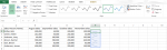
Step 3: Click on the cell where you want to insert a Sparkline and click on the Insert tab
![]()
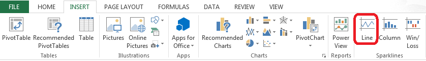
Step 4: Click on Line in the Sparklines section
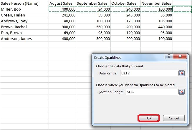
Step 5: Highlight the cells that you want to include in your Sparkline and click OK on the Sparkline creator box
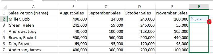
Step 5: Click on the cell with the new Sparkline and drag it down using the Fill Handle option at the bottom corner of the cell. This will create a Sparkline for each row with its corresponding data
Step 6: You can change the markers, tapes and style on your Sparkline by simply clicking on a cell with the Sparkline in it and using the options that automatically open up in the design tab
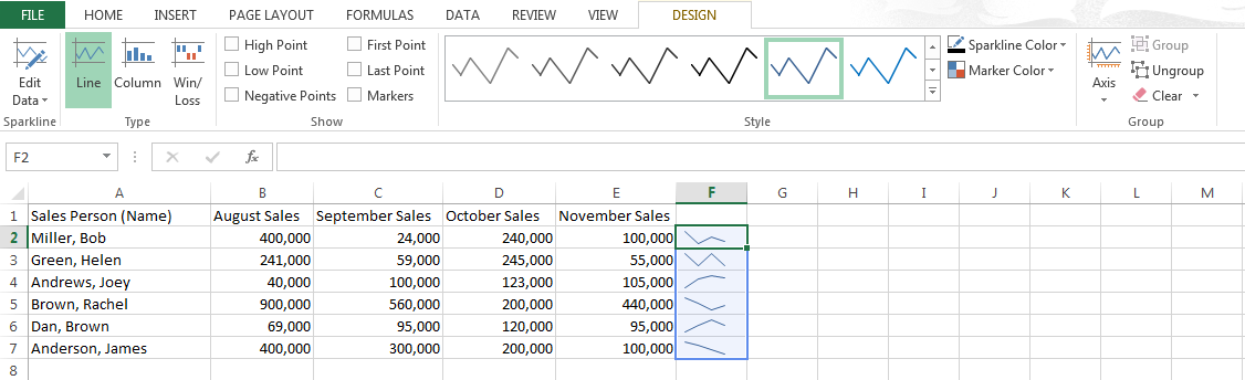
Step 7: Using the above design tab, you can mark the high points, low points and much more. You can also change the color of your Sparkline as well as edit the data that it is made up of