How to Filter Data in a Table in Excel 2013
Learning how to filter data in a table in Excel 2013 is extremely useful. If you learn this useful trick, you can sort out and view only that data which is relevant to you at any given time. This is particularly useful when you have large amounts of data and find it difficult to manage and organize it into viewable segments. If you learn how to filter data in a table in Excel 2013, you can divide your data into manageable portions. This step-by-step guide will teach you the best way how to filter data in a table in Excel 2013.
Step 1: Launch Excel 2013
Step 2: Open a document with a table
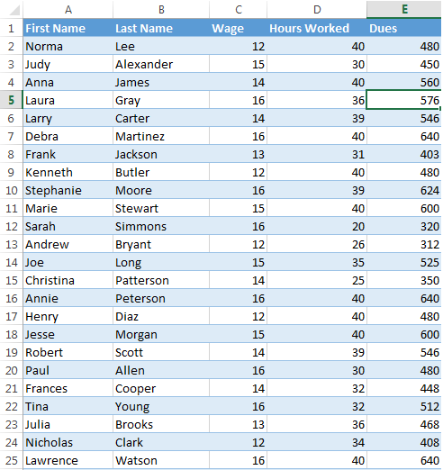
Step 3: Click anywhere on a table
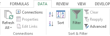
Step 4: Click on the Data tab
![]()
Step 5: Click on Filter in the Sort & Filter section
Step 6: Click on any of the arrows that appear around the top row of your table
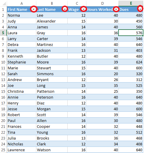
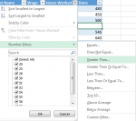
Step 7: If you want to only see employees who have worked over 35 hours, click on the arrow in the Hours Worked column. Here you can access a number of different filtering options. For this example, scroll down to Number Filters and choose Greater Than… in the side menu.

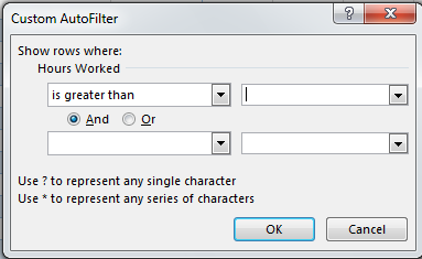
Step 8: Enter in the filtering details and click OK